Approximating inverse covariance matrices

Phew, the last time I have posted an entry to my blog was a loong time ago.. Not that there was nothing interesting to blog about, just I always delayed things. (Btw, google changed the template which eliminated the rendering of the latex formulae, not happy.. Luckily, I could change back the template..) Now, as the actual contents:

I have just read the PAMI paper "Accuracy of Pseudo-Inverse Covariance Learning-A Random Matrix Theory Analysis" by D Hoyle (IEEE T. PAMI, 2011 vol. 33 (7) pp. 1470--1481).

The paper is about pseudo-inverse covariance matrices and their analysis based on random matrix theory analysis and I can say I enjoyed this paper quite a lot.

In short, the author's point is this:
Let $d,n>0$ be integers. Let $\hat{C}$ be the sample covariance matrix of some iid data $X_1,\ldots,X_n\in \mathbb{R}^d$ based on $n$ datapoints and let $C$ be the population covariance matrix (i.e., $\hat{C}=\mathbb{E}[X_1 X_1^\top]$). Assume that $d,n\rightarrow \infty$ while $\alpha = n/d$ is kept fixed. Assume some form of "consistency" so that the eigenvalues of $C$ tend to some distribution over $[0,\infty)$. Denote by $L_{n,d} = d^{-1} \mathbb{E}[ \| C^{-1} - \hat{C}^{\dagger} \|_F^2]$ the reconstruction error of the inverse covariance matrix when one uses the pseudo-inverse.

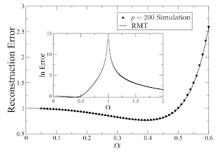
Then, $f(\alpha) := \lim_{d,n\rightarrow\infty} L_{n,d}$ will be well-defined (often). The main things is that $f$ becomes unbounded as $\alpha\rightarrow 1$ (also $\alpha\rightarrow 0$, but this is not that interesting). In fact, for $C=I$, there is an exact formula for $\alpha \rightarrow 1$:

$$f(\alpha) = \Theta(\alpha^3/(1-\alpha)^3).$$
Here is a figure that shows $f$ (on the figure $p$ denotes the dimension $d$).

Nice.

The author calls this the "peaking phenomenon": The worst case, from the point of view estimating $C^{-1}$, is when we have as many data points as is the number of dimensions (assuming full rank $C$, or this won't make sense because otherwise you could just add dummy dimensions to improve $L_{n,d}$). The explanation is that $L_{n,d}$ is just sensitive to how small the smallest positive eigenvalue of $\hat{C}$ is (this can be shown), and this smallest positive eigenvalue will become extremely small as $\alpha\rightarrow 1$ (and it does not matter whether $\alpha \rightarrow 1-$ or $\alpha\rightarrow 1+$).

Now notice that having $\alpha=0.5$ is much better than having $\alpha=1$ (for large $n,d$). Thus, there are obvious ways of improving the sample covariance estimate!

In fact, the author then suggests that in practice, assuming $n \ge d$, one should use bagging, while for $n\le d$ one should use random projections. Then he shows experimentally that this improves things though unfortunately this is shown for Fisher discriminants that uses such inverses and the demonstration for $L_{n,d}$ is lacking. He also notes that the "peaking phenomenon" can also be dealt with by other means, such as regularization where we are referred to Bickel and Levina (AoS, 2008).

Anyhow, one clear conclusion of this paper is that the pseudo-inverse must be abandoned when it comes to approximate the inverse covariance matrix. Why is this interesting? The issue of how well $C^{-1}$ can be estimated comes up naturally in regression, or even in reinforcement learning when using the projected Bellman error. And asymptotics is just a cool tool to study how things behave..