Constrained MDPs and the reward hypothesis
It's been a looong ago that I posted on this blog. But this should not mean the blog is dead. Slow and steady wins the race, right?
Anyhow, I am back and today I want to write about constrained Markovian Decision Process (CMDPs).
The post is prompted by a recent visit
of Eugene Feinberg, a pioneer of CMDPs, of our department, and also by a growing interest in CMPDs in the RL community
(see this,
this, or
this paper).
For impatient readers, a CMDP is like an MDP except that there are multiple reward functions, one of which is used to set the optimization objective, while the others are used to restrict what policies can do. Now, it seems to me that more often than not the problems we want to solve are easiest to specify using multiple objectives (in fact, this is a borderline tautology!). An example, which given our current sad situation is hard to escape, is deciding what interventions a government should apply to limit the spread of a virus while maintaining economic productivity. A perhaps less cheesy example is what interventions to apply to protect the environment, while, again, maintaining economic productivity. But we may also think of the problem of designing the software that runs an autonomous car and that must balance safety, efficiency and comfort. Or think of a robot that must maintain a success rate of achieving some task while running cheaply and smoothly.
The modest goal of of this post is to explore the relationship between CMDPs and MDPs. By definition, CMDPs are a superclass of MDPs: Every MDP is a CMDP (with no constraining reward functions). But could it be that CMDPs do not actually add much to MDPs? This relates to Rich Sutton's reward hypothesis that states
My interpretation of this hypothesis is that, given where we are now in, to maximize the speed of progress, we should focus on single-objective problems. A narrower interpretation of the hypothesis is that a single reward function (objective) suffices whatever problem we want our "intelligent agents" solve. Clearly, CMDPs go directly against this latter interpretation. But perhaps multi-objective problems can be reexpressed in terms of a single objective? Or not? The rest of this post will explain my understanding of the current state of affairs on these questions.
As it was noted before, constrained MDPs are like normal ones, except that there are multiple reward functions, say $r_0,r_1,\dots,r_n$. These are functions that map $Z\subset S \times A$ to reals. Here, $S$ is the set of states, $A$ is the set of actions and $Z$ (possibly, a strict subset of $S\times A$) determines what actions are available in each state. In particular, $Z$ is such that for each state $s\in S$, $(s,a)\in Z$ for at least one action $A$. The transition structure $P = (P_z)_{z\in Z}$ is a collection of probability distributions $P_z$ over $S$: For $z=(s,a)\in Z$, $P_z$ gives the distribution of the state that one arrives at after taking action $a$ in state $s$. For the sake of simplicity and to avoid distracting technicalities, we assume that there are finitely many states and actions.
In the discounted version of constrained MDPs, our focus in this post, one considers the total expected discounted reward under the $n+1$ reward functions to create a number of objectives. Assume for simplicity a common discount factor $0\le \gamma <1$ across all rewards. For a policy $\pi$, state $s$ and reward function $r_i$, let \[ V^\pi(r_i,s) = \mathbb{E}_s^{\pi}[\sum_{t=0}^\infty \gamma^t r_i(S_t,A_t)] \] denote the total expected discounted reward under $r_i$ collected while policy $\pi$ is followed indefinitely from state $s$. Here, $S_t$ is the state at time $t$, $A_t$ is the action at time $t$, $\mathbb{E}_s^{\pi}$ is the expectation under the probability measure $\mathbb{P}_s^\pi$ over the set of infinitely long state-action trajectories where $\mathbb{P}_s^\pi$ is induced by $P$, the policy $\pi$ (which directs what actions to take given what history), and the initial state $s$. By abusing notation, we will also use $V^\pi(r_i,\mu)$ to denote the total expected discount reward under $r_i$ when $\pi$ is started from an initial state chosen at random from $\mu$, a distribution over the states. We will also write $\mathbb{P}_\mu^\pi$ (and $\mathbb{E}_{\mu}^\pi$) to denote the probability measure over trajectories induced by $\mu$, $\pi$ and $P$ (and the underlying expectation operator, respectively).
Now, given some fixed initial state distribution $\mu$ and reals $\theta_1,\dots,\theta_n\in \mathbb{R}$, the CMDP optimization problem is to find a policy $\pi$ that maximizes $V^\pi(r_0,\mu)$ subject to the constraints $V^\pi(r_i,\mu)\ge \theta_i$, $i=1,\dots,n$: \[ \max_\pi V^\pi(r_0,\mu) \quad \text{ s.t. } \quad V^\pi(r_i,\mu) \ge \theta_i,\, i=1,\dots,n \,. \tag{$\text{CMDP}_\mu$} \] Note that here the optimization is over all possible policies. In particular, the policies can use the full history at any given stage and can also randomize. The CMDP feasibility problem is to verify whether there exists any policy that satisfies the constraints in $\text{CMDP}_\mu$. When $n=0$, we get back MDPs -- and the feasibility question becomes trivial.
An interesting and important property of MDPs is that history is not needed to act optimally. In fact, in MDPs it also holds that one can find some deterministic state-feedback policy that is uniformly optimal in the sense that it maximizes the value simultaneously over all initial distributions.
Theorem:
Parts 1,2, and 4 are from the classic book of Eitman Altman, while Part 3 is from a paper of Eugene Feinberg (the paper appeared at MOR in 2000). In what follows, I will briefly describe the reasoning behind these results, and then wrap up by describing what these results imply for the reward hypothesis. Part (5) is semi-original and while there is a sizeable literature that this part relates to, there is no obvious single reference to point to. Rest assured, I will list a number of relevant related works at the end of the post. As to the technical contents of the rest of the post, the reader will meet occupancy measures, their relationship to value functions, linear programs, Hamiltonians, Lagrangians and stochastic approximation.

The figure shows a two-state MDP; the states are marked by "L" and "R" (standing for "left" and "right"). In state "L" there are two actions: Staying in the left state ("LEFT") and moving to the right ("RIGHT"). In state "R" there is only one action available: Staying in that state ("STAY"). Transitions are deterministic. The rewards under the two reward functions $r_0$ and $r_1$ are shown next to each transition. The two reward functions agree on all transitions except the one that results in moving from left to right. In particular, under both reward functions, staying in the left state results in no reward and staying in the right state results in a reward of $+1$, while the transition from left to right incurs a reward of $+1$ under $r_0$ and it incurs the negative reward of $-1$ under $r_1$, hence, resulting in a conflict between the two rewards, as typical for constrained problems.
Forgetting for a moment about $r_1$, under $r_0$, regardless of $0\le \gamma<1$, the unique optimal policy $\pi^*$ chooses to go right in state "L". Let us, for simplicity, assume that the long-term future is discounting away: $\gamma=0$. Further, let the threshold $\theta_1$ be chosen to be zero: $\theta_1 = 0$. Since $V^{\pi^*}(r_1,L)=-1\lt 0$, $\pi^*$ is eliminated by the constraint.
Any stationary policy in this CMDP is characterized by a single number $p\in [0,1]$: The probability of choosing to stay in the left state. By abusing notation, we identify these policies with these probabilities. Similarly, we identify the initial state distributions with the probability $\beta\in [0,1]$ of starting from the left state. Then, for $p\in [0,1]$, it holds that \begin{align*} V^p(r_0,\beta) = \beta(1-p)+1-\beta\,,\\ V^p(r_1,\beta) = \beta(p-1)+1-\beta\,. \end{align*} Thus, for some $\beta\in [0,1]$, the set of feasible stationary policies are those where the value of $p$ satisfies \[ \beta(p-1)+1-\beta \ge 0 \quad \Leftrightarrow \quad p \ge \frac{2\beta-1}{\beta}\,. \] When $\beta \gt 0.5$, the valid range for $p$ is $[(2\beta-1)/\beta,1]\subsetneq [0,1]$. Thus, there is only one optimal stationary policy, which is given by the parameter $p^* = (2\beta-1)/\beta$ (this is because $V^p(r_0,\beta)$ is decreasing in $p$). Since this depends on $\beta$, there is no uniformly optimal policy among stationary policies. We also see that policies that randomize can achieve better value than policies that do not randomize. The example also shows that by restricting policies to be deterministic one can lose as much as the difference between the respective values of the best and the worst policies.
The promised relationship between values and occupancy measures is as follows: For any reward function $r$, policy $\pi$, initial state distribution $\mu$, \begin{align*} (1-\gamma) V^\pi(r,\mu) & = (1-\gamma) \sum_{t=0}^\infty \gamma^t \mathbb{E}_\mu^\pi[r(S_t,A_t)] \\ & = (1-\gamma) \sum_{t=0}^\infty \gamma^t \sum_{s,a} \mathbb{P}_\mu^\pi(S_t=s,A_t=a) r(s,a) \\ & = \langle \nu_\mu^\pi, r \rangle\,. \end{align*} Here, the last equation uses the inner product notation ($\langle f,g \rangle = \sum_z f(z) g(z)$) to emphasize that this expression is linear in both the occupancy measure and the reward. Based on the last expression, it is clear that to prove the sufficiency of stationary policies it suffices to prove that the occupancy measure of any policy $\pi$ can be replicated using the occupancy of some stationary policy.
To prove the latter, pick an arbitrary policy $\pi$ and a distribution $\mu$. We want to show that there is a stationary policy $\pi'$ such that \begin{align*} \nu_\mu^\pi(s,a) = \nu_\mu^{\pi'}(s,a), \qquad \forall (s,a)\in Z\,. \tag{ST} \end{align*} By abusing notation, define $\nu_\mu^\pi(s)=\sum_a \nu_\mu^\pi(s,a)$. Note that this is the discounted state visitation probability distribution induced by $\mu$ and $\pi$. (In fact, $\nu_\mu^\pi(s) = (1-\gamma) V^\pi_\mu(e_s,s)$ where $e_s$ is the binary-valued reward function that rewards taking any action in state $s$.) Now, define the stationary policy $\pi'$ as follows: For states $s$ such that $\nu_\mu^\pi(s)\ne 0$, we let \begin{align*} \pi'(a|s) = \frac{\nu_\mu^\pi(s,a)}{\nu_\mu^\pi(s)}\,, \end{align*} while for states with $\nu_\mu^\pi(s)=0$, we pick any probability distribution.
We will now show that $\nu_\mu^\pi(s) = \nu_\mu^{\pi'}(s)$ for any state $s$, which immediately implies $(\text{ST})$. Recall that $P_{s,a}(s')$ is the probability of transitioning to state $s'$ when action $a$ is taken in state $s$. Define $P^{\pi'}$ by $P_s^{\pi'}(s') = \sum_{a} \pi'(a|s) P_{s,a}(s')$. This is thus the probability of transitioning to state $s'$ when policy $\pi'$ is followed from state $s$ for one time step. Now, \begin{align*} \nu_\mu^\pi(s) & = (1-\gamma) \sum_{t\ge 0} \gamma^t \mathbb{P}_\mu^\pi(S_t=s) \\ & = (1-\gamma) \mu(s) + (1-\gamma) \gamma \sum_{t\ge 0} \gamma^t \mathbb{P}_\mu^\pi(S_{t+1}=s) \\ %& = (1-\gamma) \mu(s) % + \gamma (1-\gamma) \sum_{t\ge 0} \gamma^t % \sum_{s',a} \mathbb{P}_\mu^\pi(S_t=s',A_t=a) P_{s',a}(s) \\ & = (1-\gamma) \mu(s) + \gamma \sum_{s',a} \left\{ (1-\gamma) \sum_{t\ge 0} \gamma^t \mathbb{P}_\mu^\pi(S_t=s',A_t=a) \right\} P_{s',a}(s) \\ & = (1-\gamma) \mu(s) + \gamma \sum_{s',a} \nu_\mu^\pi(s',a) P_{s',a}(s) \\ & = (1-\gamma) \mu(s) + \gamma \sum_{s'} \nu_\mu^\pi(s') P^{\pi'}_{s'}(s)\,. \tag{**} \end{align*} Fixing a canonical ordering over the states, we can view $(\nu_\mu^\pi(s))_{s}$ as a row-vector and $(P^{\pi'}_{s'}(s))_{s',s}$ as a matrix. Then, the above identity can be written in the short form \[ \nu_\mu^\pi = (1-\gamma) \mu + \gamma \nu_\mu^\pi P^{\pi'}\,. \] Reordering, and solving for $\nu_\mu^\pi$, we get, \[ \nu_\mu^\pi = (1-\gamma) \mu (I - \gamma P^{\pi'})^{-1} = \nu_\mu^{\pi'}, \] where the second equality follows from $(**)$ and noting that by $(*)$, $\nu^{\pi'}(s,a)= \pi'(a|s) \nu^{\pi'}(s)$ (that the inverse of $I-\gamma P^{\pi'}$ exists follows from that for arbitrary $z$, $x \mapsto z + \gamma x P^{\pi'}$ defines a max-norm contraction). Together with our previous argument, this finishes the proof that stationary policies are sufficient in CMDPs.
Theorem:
Checking feasibility in CMDPs among deterministic policies is NP-hard.
But why would one care about deterministic policies? We already know that the best deterministic policies may be arbitrarily worse than the best stationary policy. Deterministic policies are still not completely out because in many applications randomization is just too hard to sell: If every time a customer comes to a website, a dice decides what they see, questions of accountability, reproducibility and explainability will inevitable arise. The same holds for many other engineering applications, such as autonomous driving. While reproducibility could be mitigated by using carefully controlled pseudorandom numbers, accountability and explainability remain a problem. Assuming that this is a convincing argument, how does it happen that feasibility checking among deterministic policies is NP-hard?
The construction to prove this claim is based on a reduction to the Hamiltonian cycles problem. Recall that the Hamiltonian cycle problem is to check whether there exists a cycle in a (say) directed graph that visits every vertex exactly once. Also recall that this is one of the classic NP-complete problems. The reduction is based on the following idea: Given a directed graph, we construct a Markov transition structure whose state space is the set of vertices, the set of admissible actions at a given state $s$ are the outgoing edges at the vertex $s$, with the transitions deterministically moving along the corresponding edge. In this graph, every Hamiltonian cycle $H$ gives rise to a deterministic policy that at a state $s$ picks the edge that is included in the cycle $H$.
Now, fix any state (vertex) $s_0$ and define the reward $r$ so that every transition out of state $s_0$ gives a unit reward and there are no other rewards: \[ r(s',a) = \begin{cases} 1, & \text{ if } s'=s_0\,;\\ 0, & \text{ otherwise}\,. \end{cases} \] If there are $N$ states (vertices), there is a Hamiltonian cycle $H$ and $\pi$ is the deterministic policy corresponding to this cycle, then \[ V^\pi(r,s_0) = 1 + \gamma^N + \gamma^{2N} + \dots = \frac{1}{1-\gamma^N}\,. \tag{H} \] The proposed problem is then as follows: \begin{align*} \textit{Check whether there exists a deterministic policy }\pi \textit{ such that (H) holds}. \tag{CC} \end{align*} For the sake of specificity, from now on we let $\gamma = 1/2$.
To see why (CC) is sufficient for the reduction, suppose that $\pi$ is a deterministic policy that satisfies (H). Since $\pi$ is deterministic, when started from $s_0$, it generates a deterministic sequence of states $s_0,s_1,\dots$. Either $s_0$ occurs a single time in this sequence ("$s_0$ is transient"), or it appears infinitely many times. If it appears a single time, $V^\pi(r,s_0) = 1$, which contradicts (H). Thus, $s_0$ must appear infinitely many times. Let $m$ be the smallest positive integer such that $s_m=s_0$. Clearly then $V^\pi(r,s_0) = 1/(1-\gamma^m)$. Hence, if (H) holds then $m=n$. It is also clear that $(s_1,\dots,s_m)$ does not have duplicates because then $s_0$ would need to be transient, which we have already ruled out. Hence, all states are visited exactly once in the sequence $s_0,s_1,\dots,s_{m-1}=s_{n-1}$, which means that this sequence defines a Hamiltonian cycle.
To finish, note that $V^\pi(r,s_0) = 1/(1-\gamma^n)$ is equivalent to $V^\pi(r,s_0)\ge 1/(1-\gamma^n)$ and $V^{\pi}(-r,s_0) \ge -1/(1-\gamma^n)$, thus showing that checking feasibility among deterministic policies with $r_1 = r$, $r_2 = -r$ and respective thresholds $1/(1-\gamma^n)$, $-1/(1-\gamma^n)$ is NP-hard. Since with $\gamma=1/2$, these thresholds are also of polynomial length in the size $n$ of the input, the proof is finished.
As to whether hardness applies to feasibility testing among stationary policies, first note that the set of occupancy measures can be described as a subset of $\mathbb{R}^Z$ that satisfies $|S|+1$ linear constraints. Indeed, our previous argument shows that for arbitrary $\pi$ and $\mu$, \begin{align*} \sum_a \nu_\mu^\pi(s,a) = (1-\gamma)\mu(s) + \gamma \sum_{s',a'} \nu_\mu^\pi(s',a') P_{s',a'}(s)\,. \end{align*} It follows that the set $X_\gamma$ of such occupancy measures satisfies \begin{align*} X_\gamma & \subset \{ x \in [0,\infty)^Z \,:\, \sum_a x(s,a)=(1-\gamma)\mu(s) + \gamma \sum_{s',a'} x(s',a') P_{s',a'}(s), \forall s\in S \}\,. \end{align*} In fact, reusing the argument used in Part (2), it is not hard to show that this display holds with equality. Now, the feasibility problem is to decide whether the set \[ F = \{ x\in X_\gamma \,:\, \langle x,r_i \rangle \ge (1-\gamma) \theta_i, i=1,\dots,n \} \] is empty. Clearly, this is also a set that is described by $|S|+1+n$ linear constraints. Hence, checking whether this set is empty is a linear feasibility problem. Linear feasibility problems can be solved in polynomial time -- assuming that the feasibility problem is well-conditioned. But is there a guarantee that the above feasibility problem is well-conditioned? When $n=1$, the answer is yes: We can just consider the single-objective MDP and solve it in polynomial time. If the objective is above $\theta_1$, we return with "Yes, the problem is feasible", otherwise we return with "No". The situation is different when feasibility under a number of different discount factors is considered:
Theorem (Feinberg, 2000):
Checking feasibility for CMDPs with $m$ states and $2m-1$ constraints with distinct discount factors is NP-hard.
One possibility is to fold the extra value constraints into the optimization objective. For this, introduce the Lagrangian function \[ L(x,\lambda) = - \langle x, r_0 \rangle + \sum_i \lambda_i ((1-\gamma) \theta_i - \langle x,r_i \rangle)\,, \] where $\lambda = (\lambda_i)_i$ are nonnegative reals, the so-called Lagrangian multipliers. Clearly, if $x$ satisfies the value constraints in $(\text{CMDP}_\mu)$ then $\sup_{\lambda\ge 0} L(x,\lambda) = - \langle x, r_0 \rangle$, while if it does not satisfy them then $\sup_{\lambda\ge 0} L(x,\lambda)=\infty$. Hence, the CMDP problem is equivalent to solving \begin{align*} \min_{x\in X_\gamma} \max_{\lambda \ge 0} L(x,\lambda) \quad \tag{MM} \end{align*} in $x$. For a fixed $x$, let $\lambda_*(x)$ denote a maximizer of $L(x,\cdot)$ over $[0,\infty]^n$ (explicitly allowing for $\lambda_i(x)=\infty$). If $x^*$ is the solution to the above problem, by definition $L(x^*,\lambda_*(x^*))\le L(x,\lambda_*(x^*))$. The tempting conclusion then is that if $\lambda^* = \lambda_*(x^*)$ was given then it will be sufficient to solve the minimization problem \[ \min_{x\in X_\gamma} L(x,\lambda^*)\,. \] This would be a great simplification of the CMDP problem, as this optimization problem corresponds to a single-objective MDP problem with reward function \[ r = r_0 + \sum_{i=1}^n \lambda_i^* r_i\,. \] One view of this is that the optimal Lagrangian multiplier choose the right conversion factors to "merge" the multiple rewards into a single reward.
Unfortunately, this argument is seriously flawed. Indeed, if it was sufficient to find a minimizer of $x \mapsto L(x,\lambda^*)$ then, given that we are in an MDP, this minimizer could always be chosen to be induced by some deterministic policy. However, such a policy cannot be optimal in the original CMDP if in there all deterministic policies are suboptimal! In Part (1), we saw an example of such an CMDP. Simple scalarization using optimal Lagrangian multipliers does not work.
The root of the problem is that while the solution $x^*$ of the CMDP problem is indeed one of the minimizers, the function $x \mapsto L(x,\lambda^*)$ will in general have many other minimizers (such as the ones that underlie deterministic policies!), and there is no guarantee that these minimizers would also solve the original problem. In fact, when $x^*$ corresponds to a non-deterministic policy, the set $\{ x\in X_\gamma\,:\, L(x,\lambda^*)=\min_{y\in X_\gamma} L(y,\lambda^*) \}$ will have infinitely many elements (in fact, we can always find a nontrivial line segment in this set).
To build up our intuition about what is happening, let us take a step back and just think a little bit about min-max problems (after all, with our Lagrangian, the CMDP problem became a min-max problem). For the sake of specificity, consider the game of Rock-Paper-Scissors. This is a game between two players (say, Alice and Bob), where each player needs to choose, simultaneously, one of rock, paper or scissors. Paper beats rock, scissor beats paper, and rock beats scissor. The player who loses pays one "Forint" to the other player. In this situation, the equilibrium strategy, for both players, is to choose an action uniformly at random. Now, if Alice knows for sure that Bob plays uniformly at random (suggestively, $\lambda_1^* = \lambda_2^* = \lambda_3^* = 1/3$), then Alice will achieve the same expected winnings (zero) using any strategy! But if Alice chose anything but the uniform strategy, Bob could reoptimize their strategy (deviating from $\lambda^*$!) and could end up with a positive expected return. So Alice should better stick to the uniform strategy; the only strategy that leaves no room for Bob to exploit Alice.
Similarly, in CMDPs it is not sufficient to find just any minimizer of $L(x,\lambda^*)$, but one needs to find a minimizer such that the value would not move even if $\lambda^*$ was reoptimized! As noted above, in general, $\lambda^*$ will in fact be such that there will be infinitely many minimizers of $L(\cdot,\lambda^*)$.
To introduce this theorem, we need some extra notation. In what follows we use $L_x'$ ($L_\lambda'$) to denote the partial derivative of $L=L(x,\lambda)$ with respect to $x$ (respectively, $\lambda$). The interested reader can explore some of the generalizations of this theorem on Wikipedia. For the astute reader, we note in advance, that its conditions will not be satisfied for our $L$ as defined above; but the theorem is still useful to motivate the algorithm that we want to introduce.
Recall that $\lambda_*(x)$ is the maximizer of $\lambda \mapsto L(x,\lambda)$. Theorem (John M. Danskin):
Let $\Phi(x) = L(x,\lambda_*(x))$. If $\lambda_*(x)$ is in $(0,\infty)^n$ and is differentiable, and both $L_x'$ and $L_\lambda'$ exist then $\Phi$ is also differentiable and $\nabla \Phi(x) = L'_x(x,\lambda_*(x))$.
Proof: Since $\lambda_*(x)\in (0,\infty)^n$, it is an unconstrained maximizer of $L(x,\cdot)$ and thus by the first-order optimality condition for extrema of differentiable functions, $L_\lambda'(x,\lambda_*(x))=0$. Hence, $\nabla \Phi(x) = L'_x(x,\lambda_*(x)) + L'_\lambda(x,\lambda_*(x)) \lambda_*'(x) = L'_x(x,\lambda_*(x))$.
Q.E.D.
By this theorem, the ordinary differential equation \[ \dot{x} = - L_x'(x,\lambda_*(x)) \tag{XU} \] describes a dynamics that converges to a minimizer of $\Phi(x)$ as long as along the trajectories we can ensure that $\lambda_*(x)$ is inside $(0,\infty)^n$ (to stay inside $X_\gamma$, one also needs to add projections, but for now let us just sweep this under the rug). This is all good, but how would we know $\lambda_*(x)$? For a given fixed value of $x$, one can of course use a gradient flow \[ \dot{\lambda} = L_\lambda'(x,\lambda)\, \tag{LU} \] which, under mild regularity conditions, guarantees that $\lim_{t\to\infty} \lambda(t)=\lambda_*(x)$ regardless of $x$. The idea is then to put the two dynamics together, making the update of $\lambda$ work on "faster" timescale than the update of $x$: \begin{align*} \dot{x} & = - \epsilon L_x'(x,\lambda)\,, \\ \dot{\lambda} & = L_\lambda'(x,\lambda) \end{align*} for $\epsilon$ "infinitesimally small". This must sound crazy! Will this, for example, make the updates infinitely slow? And what happens when $\lambda_*(x)$ is not finite?
Interestingly, a simple Euler discretization, with decreasing step-sizes, one that is often used anyways when only a noisy "estimate" of the gradients $L_x'$ and $L_\lambda'$ are available, addresses all the concerns! We just have to think about the update of $\lambda$ being indefinitely faster than that of $x$, rather than thinking of $x$ being updated indefinitely slower than $\lambda$. This results in the updates \begin{align*} x_{k+1}-x_k &= - a_k (L_x'(x_k,\lambda_k)+W_k) \,,\\ \lambda_{k+1} - \lambda_k &= b_k (L_\lambda'(x_k,\lambda_k)+U_k)\,, \end{align*} where the positive stepsize sequences $(a_k)_k$, $(b_k)_k$ are such that $a_k \ll b_k$ and both converge to zero not too fast and not too slow, and where $W_k$ and $U_k$ are zero-mean noise sequences. This is what is known as a two-timescale stochastic approximation update. In particular, the timescale separation happens together with "convergence in the limit" if the stepsizes are chosen to satisfy \begin{align*} a_k = o(b_k) \quad k \to \infty\,,\\ \sum_k a_k = \sum_k b_k = \infty, \quad \sum_k a_k^2<\infty, \sum_k b_k^2 <\infty\,. \end{align*} This may make some worry about that $a_k$ will be too small and thus $x_k$ may converge slowly. The trick is to make $b_k$ larger rather than making $a_k$ smaller. For example, we can use $a_k = c/k$ if it is paired with $b_k = c/k^{0.5+\gamma}$ for $0<\gamma<0.5$. This makes the $\lambda_k$ iterates "more noisy", but the $x_k$ updates can smooth this noise out and since now $\lambda_k$ will also converge a little faster than usual, the $x_k$ can converge at the usual statistical rate of $1/\sqrt{k}$. The details are not trivial and a careful analysis is necessary to show that these ideas work and in fact I have not seen a complete analysis of this approach. To convince the reader that these ideas will actually work, I include a figure that shows how the iterates evolve in time in a simple, noiseless case. In fact, I include two figures: One when $x$ is updated on the slow timescale (the approach proposed here) but also the one when $\lambda$ is updated on the slow timescale. Surprisingly, this second approach is the one that makes an appearance in pretty much all the CMDP learning papers that use a two-timescale approach. As suggested by our argument of Part 3, and confirmed by the simulation results shown, this approach just cannot work: The $x$ variable will keep oscillating between its extreme values (representing deterministic policies).
Simulation results for the case when there is a single state, two actions.
If $x$ is the probability of taking the first action, the payoff under $r_0$ is $-x$ (e.g., $r_0(1)=-1$, $r_0(2)=0$). The payoff under $r_1$ is $x$ and the respective threshold is $0.5$. Altogether, this results in the constrained optimization problem "$\min_{x\in [0,1]} x$ subject to $x\ge 1/2$". The Lagrangian is $L(x,\lambda) = x + \lambda_*(1/2-x)$. The left-hand subfigure shows $x$ and $\lambda$ as a function of the number of updates when the stepsizes are $1/k$ ($1/\sqrt{k}$) for updating $x$ (respectively, $\lambda$). The stepsizes are reversed for the right-hand side figure. As it is obvious from the figures, only the variable that is updated on the slow timescale converges to its optimal value.
As the figures on the left-hand side attest, the algorithm works, though given how simple the example considered is, the oscillations and the slow convergence are rather worrysome. Readers familiar with the optimization literature will recognize this as a problem that has been long recognized in that literature, where various remedies have also been proposed. However, rather than exploring these here (for the curious reader, we give some pointers to the literature at the end of the post), let us turn to addressing the next major limitation of the approach presented so far, which is that in its current form the algorithm needs to maintain an occupancy measure over the states, which is usually quite problematic.
A trivial way to avoid representing occupancy measures is if search directly in a smoothly parameterized policy class. Let $\pi_\rho = \pi_\rho(a|s)$ be such a policy parameterization, where $\rho$ lives in some finite dimensional vector space. Then, we can write the Lagrangian \begin{align*} L(\rho,\lambda) & = - (1-\gamma) V^{\pi_\rho}(r_0,\mu) - \sum_i \lambda_i ((1-\gamma) V^{\pi_\rho}( r_i, \mu )-(1-\gamma)\theta_i) \\ & = - (1-\gamma) V^{\pi_\rho}\left(r_0+\sum_i \lambda_i r_i, \mu \right)+ (1-\gamma) \sum_i \lambda_i \theta_i\,, \end{align*} and our previous reasoning goes through without any changes. The gradient of $L$ with respect to $\rho$ can then be obtained using any of the "policy search" approaches available in the literature: As long as we can argue that these updates follow the gradient $L_\rho'(\rho,\lambda)$, we expect that the algorithm will find a locally optimal policy, which satisfies the value constraints.
Finally, to see what it takes to update the Lagrangian multipliers $(\lambda_i)_i$, we calculate \[ \frac{\partial}{\partial \lambda_i} L(\rho,\lambda) = (1-\gamma)\theta_i-(1-\gamma) V^{\pi_\rho}( r_i, \mu )\,. \] That is, $\lambda_i$ will be increased if the $i$th constraint is violated, while it will be decreased otherwise. Reassuringly, this makes intuitive sense. The update also tells us that the full algorithm will need to estimate the value of the policy to be updated under all the reward functions $r_i$.
Stepping back from the calculations a little, what saved the day here? Why could we reuse policy search algorithms to search for the solution of a constrained problem whereas in Part (4) we suggested that finding the optimal Lagrangian $\lambda^*$ and then solving the resulting minimization problem will not work? The magic is due to the use of gradient descent but the unsung hero is Danskin's theorem, which suggests that updating the parameters by following the partial derivative is a sensible choice.
Of course, as any general arvice, this rule works also best when it is applied with moderation. In particular, the advice does not mean that we should never work on new problems, or that we should necessarily shy away from "big, hairy problems". Good research always dances on the boundary of what is possible.
As to specific research questions that one can ask, it appears that while there has been some work on developing algorithms for CMDPs, much remains to be done. Example of open questions include but are not limited to the following:
For impatient readers, a CMDP is like an MDP except that there are multiple reward functions, one of which is used to set the optimization objective, while the others are used to restrict what policies can do. Now, it seems to me that more often than not the problems we want to solve are easiest to specify using multiple objectives (in fact, this is a borderline tautology!). An example, which given our current sad situation is hard to escape, is deciding what interventions a government should apply to limit the spread of a virus while maintaining economic productivity. A perhaps less cheesy example is what interventions to apply to protect the environment, while, again, maintaining economic productivity. But we may also think of the problem of designing the software that runs an autonomous car and that must balance safety, efficiency and comfort. Or think of a robot that must maintain a success rate of achieving some task while running cheaply and smoothly.
The modest goal of of this post is to explore the relationship between CMDPs and MDPs. By definition, CMDPs are a superclass of MDPs: Every MDP is a CMDP (with no constraining reward functions). But could it be that CMDPs do not actually add much to MDPs? This relates to Rich Sutton's reward hypothesis that states
"That all of what we mean by goals and purposes can be well thought of as maximization of the expected value of the cumulative sum of a received scalar signal (reward)."
My interpretation of this hypothesis is that, given where we are now in, to maximize the speed of progress, we should focus on single-objective problems. A narrower interpretation of the hypothesis is that a single reward function (objective) suffices whatever problem we want our "intelligent agents" solve. Clearly, CMDPs go directly against this latter interpretation. But perhaps multi-objective problems can be reexpressed in terms of a single objective? Or not? The rest of this post will explain my understanding of the current state of affairs on these questions.
Constrained MDPs: Definitions
I will assume that readers are familiar with MDPs. Readers who need a refresher on MDP definitions and concepts (policies, etc.) can scroll to the bottom of the post and then come back. Why to use MDPs should be the topic of another post; for now the reader is asked to accept that we start with MDPs.As it was noted before, constrained MDPs are like normal ones, except that there are multiple reward functions, say $r_0,r_1,\dots,r_n$. These are functions that map $Z\subset S \times A$ to reals. Here, $S$ is the set of states, $A$ is the set of actions and $Z$ (possibly, a strict subset of $S\times A$) determines what actions are available in each state. In particular, $Z$ is such that for each state $s\in S$, $(s,a)\in Z$ for at least one action $A$. The transition structure $P = (P_z)_{z\in Z}$ is a collection of probability distributions $P_z$ over $S$: For $z=(s,a)\in Z$, $P_z$ gives the distribution of the state that one arrives at after taking action $a$ in state $s$. For the sake of simplicity and to avoid distracting technicalities, we assume that there are finitely many states and actions.
In the discounted version of constrained MDPs, our focus in this post, one considers the total expected discounted reward under the $n+1$ reward functions to create a number of objectives. Assume for simplicity a common discount factor $0\le \gamma <1$ across all rewards. For a policy $\pi$, state $s$ and reward function $r_i$, let \[ V^\pi(r_i,s) = \mathbb{E}_s^{\pi}[\sum_{t=0}^\infty \gamma^t r_i(S_t,A_t)] \] denote the total expected discounted reward under $r_i$ collected while policy $\pi$ is followed indefinitely from state $s$. Here, $S_t$ is the state at time $t$, $A_t$ is the action at time $t$, $\mathbb{E}_s^{\pi}$ is the expectation under the probability measure $\mathbb{P}_s^\pi$ over the set of infinitely long state-action trajectories where $\mathbb{P}_s^\pi$ is induced by $P$, the policy $\pi$ (which directs what actions to take given what history), and the initial state $s$. By abusing notation, we will also use $V^\pi(r_i,\mu)$ to denote the total expected discount reward under $r_i$ when $\pi$ is started from an initial state chosen at random from $\mu$, a distribution over the states. We will also write $\mathbb{P}_\mu^\pi$ (and $\mathbb{E}_{\mu}^\pi$) to denote the probability measure over trajectories induced by $\mu$, $\pi$ and $P$ (and the underlying expectation operator, respectively).
Now, given some fixed initial state distribution $\mu$ and reals $\theta_1,\dots,\theta_n\in \mathbb{R}$, the CMDP optimization problem is to find a policy $\pi$ that maximizes $V^\pi(r_0,\mu)$ subject to the constraints $V^\pi(r_i,\mu)\ge \theta_i$, $i=1,\dots,n$: \[ \max_\pi V^\pi(r_0,\mu) \quad \text{ s.t. } \quad V^\pi(r_i,\mu) \ge \theta_i,\, i=1,\dots,n \,. \tag{$\text{CMDP}_\mu$} \] Note that here the optimization is over all possible policies. In particular, the policies can use the full history at any given stage and can also randomize. The CMDP feasibility problem is to verify whether there exists any policy that satisfies the constraints in $\text{CMDP}_\mu$. When $n=0$, we get back MDPs -- and the feasibility question becomes trivial.
An interesting and important property of MDPs is that history is not needed to act optimally. In fact, in MDPs it also holds that one can find some deterministic state-feedback policy that is uniformly optimal in the sense that it maximizes the value simultaneously over all initial distributions.
Main result
To jump into the middle of things, I state a "theorem" that lists some of the ways in which CMDPs are different from MDPs. To state this theorem, recall that a policy is called stationary if it uses state-feedback, but can also randomize. Stationary policies are preferred as they have a simple structure: The policy does not need to remember the past; i.e., it is memoryless.Theorem:
- Uniformly optimal stationary policies may not exist and optimal policies may need to randomize;
- Stationary policies suffice in CMDPs;
- Feasibility can be hard to check in CMDPs;
- CMDPs can be recasted as linear programs, but they cannot be casted as MDPs with identical state-action spaces.
- Gradient algorithms designed for MDPs can be made to work for CMDPs.
Parts 1,2, and 4 are from the classic book of Eitman Altman, while Part 3 is from a paper of Eugene Feinberg (the paper appeared at MOR in 2000). In what follows, I will briefly describe the reasoning behind these results, and then wrap up by describing what these results imply for the reward hypothesis. Part (5) is semi-original and while there is a sizeable literature that this part relates to, there is no obvious single reference to point to. Rest assured, I will list a number of relevant related works at the end of the post. As to the technical contents of the rest of the post, the reader will meet occupancy measures, their relationship to value functions, linear programs, Hamiltonians, Lagrangians and stochastic approximation.
Part 1: Lack of uniformly optimal stationary policies and the need for randomization
This part only needs an example. This is best done graphically:
Figure: 2-state MDP example for illustrating CMDPs
The figure shows a two-state MDP; the states are marked by "L" and "R" (standing for "left" and "right"). In state "L" there are two actions: Staying in the left state ("LEFT") and moving to the right ("RIGHT"). In state "R" there is only one action available: Staying in that state ("STAY"). Transitions are deterministic. The rewards under the two reward functions $r_0$ and $r_1$ are shown next to each transition. The two reward functions agree on all transitions except the one that results in moving from left to right. In particular, under both reward functions, staying in the left state results in no reward and staying in the right state results in a reward of $+1$, while the transition from left to right incurs a reward of $+1$ under $r_0$ and it incurs the negative reward of $-1$ under $r_1$, hence, resulting in a conflict between the two rewards, as typical for constrained problems.
Forgetting for a moment about $r_1$, under $r_0$, regardless of $0\le \gamma<1$, the unique optimal policy $\pi^*$ chooses to go right in state "L". Let us, for simplicity, assume that the long-term future is discounting away: $\gamma=0$. Further, let the threshold $\theta_1$ be chosen to be zero: $\theta_1 = 0$. Since $V^{\pi^*}(r_1,L)=-1\lt 0$, $\pi^*$ is eliminated by the constraint.
Any stationary policy in this CMDP is characterized by a single number $p\in [0,1]$: The probability of choosing to stay in the left state. By abusing notation, we identify these policies with these probabilities. Similarly, we identify the initial state distributions with the probability $\beta\in [0,1]$ of starting from the left state. Then, for $p\in [0,1]$, it holds that \begin{align*} V^p(r_0,\beta) = \beta(1-p)+1-\beta\,,\\ V^p(r_1,\beta) = \beta(p-1)+1-\beta\,. \end{align*} Thus, for some $\beta\in [0,1]$, the set of feasible stationary policies are those where the value of $p$ satisfies \[ \beta(p-1)+1-\beta \ge 0 \quad \Leftrightarrow \quad p \ge \frac{2\beta-1}{\beta}\,. \] When $\beta \gt 0.5$, the valid range for $p$ is $[(2\beta-1)/\beta,1]\subsetneq [0,1]$. Thus, there is only one optimal stationary policy, which is given by the parameter $p^* = (2\beta-1)/\beta$ (this is because $V^p(r_0,\beta)$ is decreasing in $p$). Since this depends on $\beta$, there is no uniformly optimal policy among stationary policies. We also see that policies that randomize can achieve better value than policies that do not randomize. The example also shows that by restricting policies to be deterministic one can lose as much as the difference between the respective values of the best and the worst policies.
Part 2: Sufficiency of stationary policies
First, let us clarify the meaning of sufficiency: we call a set of policies sufficient if for any CMDP, the set contains an optimal policy. The sufficiency of stationary policies will follow from a close correspondence between value functions and occupancy measures and that stationary policies "span" the set of all occupancy measures. But what are these occupancy measures? Given an arbitrary policy $\pi$ and initial state distribution $\mu$, for state-action pair $(s,a)\in Z$, let \[ \nu_\mu^\pi(s,a) = (1-\gamma) \sum_{t=0}^\infty \gamma^t \mathbb{P}_\mu^\pi( S_t = s,A_t = a)\,. \tag{*} \] We call $\nu_\mu^\pi$ the discounted normalized occupancy measure underlying $\pi$ and $\mu$: It is the mesure that counts the expected discounted number of "visits" of the individual admissible state-action pairs. The normalizer $(1-\gamma)$ makes $\nu_\mu^\pi$ a probability measure: $\sum_{s,a} \nu_\mu^\pi(s,a)=1$. To save space, in what follows, we will shorten the name of $\nu_\mu^\pi$ and will just say that it is an occupancy measure.The promised relationship between values and occupancy measures is as follows: For any reward function $r$, policy $\pi$, initial state distribution $\mu$, \begin{align*} (1-\gamma) V^\pi(r,\mu) & = (1-\gamma) \sum_{t=0}^\infty \gamma^t \mathbb{E}_\mu^\pi[r(S_t,A_t)] \\ & = (1-\gamma) \sum_{t=0}^\infty \gamma^t \sum_{s,a} \mathbb{P}_\mu^\pi(S_t=s,A_t=a) r(s,a) \\ & = \langle \nu_\mu^\pi, r \rangle\,. \end{align*} Here, the last equation uses the inner product notation ($\langle f,g \rangle = \sum_z f(z) g(z)$) to emphasize that this expression is linear in both the occupancy measure and the reward. Based on the last expression, it is clear that to prove the sufficiency of stationary policies it suffices to prove that the occupancy measure of any policy $\pi$ can be replicated using the occupancy of some stationary policy.
To prove the latter, pick an arbitrary policy $\pi$ and a distribution $\mu$. We want to show that there is a stationary policy $\pi'$ such that \begin{align*} \nu_\mu^\pi(s,a) = \nu_\mu^{\pi'}(s,a), \qquad \forall (s,a)\in Z\,. \tag{ST} \end{align*} By abusing notation, define $\nu_\mu^\pi(s)=\sum_a \nu_\mu^\pi(s,a)$. Note that this is the discounted state visitation probability distribution induced by $\mu$ and $\pi$. (In fact, $\nu_\mu^\pi(s) = (1-\gamma) V^\pi_\mu(e_s,s)$ where $e_s$ is the binary-valued reward function that rewards taking any action in state $s$.) Now, define the stationary policy $\pi'$ as follows: For states $s$ such that $\nu_\mu^\pi(s)\ne 0$, we let \begin{align*} \pi'(a|s) = \frac{\nu_\mu^\pi(s,a)}{\nu_\mu^\pi(s)}\,, \end{align*} while for states with $\nu_\mu^\pi(s)=0$, we pick any probability distribution.
We will now show that $\nu_\mu^\pi(s) = \nu_\mu^{\pi'}(s)$ for any state $s$, which immediately implies $(\text{ST})$. Recall that $P_{s,a}(s')$ is the probability of transitioning to state $s'$ when action $a$ is taken in state $s$. Define $P^{\pi'}$ by $P_s^{\pi'}(s') = \sum_{a} \pi'(a|s) P_{s,a}(s')$. This is thus the probability of transitioning to state $s'$ when policy $\pi'$ is followed from state $s$ for one time step. Now, \begin{align*} \nu_\mu^\pi(s) & = (1-\gamma) \sum_{t\ge 0} \gamma^t \mathbb{P}_\mu^\pi(S_t=s) \\ & = (1-\gamma) \mu(s) + (1-\gamma) \gamma \sum_{t\ge 0} \gamma^t \mathbb{P}_\mu^\pi(S_{t+1}=s) \\ %& = (1-\gamma) \mu(s) % + \gamma (1-\gamma) \sum_{t\ge 0} \gamma^t % \sum_{s',a} \mathbb{P}_\mu^\pi(S_t=s',A_t=a) P_{s',a}(s) \\ & = (1-\gamma) \mu(s) + \gamma \sum_{s',a} \left\{ (1-\gamma) \sum_{t\ge 0} \gamma^t \mathbb{P}_\mu^\pi(S_t=s',A_t=a) \right\} P_{s',a}(s) \\ & = (1-\gamma) \mu(s) + \gamma \sum_{s',a} \nu_\mu^\pi(s',a) P_{s',a}(s) \\ & = (1-\gamma) \mu(s) + \gamma \sum_{s'} \nu_\mu^\pi(s') P^{\pi'}_{s'}(s)\,. \tag{**} \end{align*} Fixing a canonical ordering over the states, we can view $(\nu_\mu^\pi(s))_{s}$ as a row-vector and $(P^{\pi'}_{s'}(s))_{s',s}$ as a matrix. Then, the above identity can be written in the short form \[ \nu_\mu^\pi = (1-\gamma) \mu + \gamma \nu_\mu^\pi P^{\pi'}\,. \] Reordering, and solving for $\nu_\mu^\pi$, we get, \[ \nu_\mu^\pi = (1-\gamma) \mu (I - \gamma P^{\pi'})^{-1} = \nu_\mu^{\pi'}, \] where the second equality follows from $(**)$ and noting that by $(*)$, $\nu^{\pi'}(s,a)= \pi'(a|s) \nu^{\pi'}(s)$ (that the inverse of $I-\gamma P^{\pi'}$ exists follows from that for arbitrary $z$, $x \mapsto z + \gamma x P^{\pi'}$ defines a max-norm contraction). Together with our previous argument, this finishes the proof that stationary policies are sufficient in CMDPs.
Part 3: Feasibility can be hard
This claim is based on a connection between Hamiltonian cycles and CMDPs. For brevity, call deterministic state-feedback policies "deterministic". We have the following theorem:Theorem:
Checking feasibility in CMDPs among deterministic policies is NP-hard.
But why would one care about deterministic policies? We already know that the best deterministic policies may be arbitrarily worse than the best stationary policy. Deterministic policies are still not completely out because in many applications randomization is just too hard to sell: If every time a customer comes to a website, a dice decides what they see, questions of accountability, reproducibility and explainability will inevitable arise. The same holds for many other engineering applications, such as autonomous driving. While reproducibility could be mitigated by using carefully controlled pseudorandom numbers, accountability and explainability remain a problem. Assuming that this is a convincing argument, how does it happen that feasibility checking among deterministic policies is NP-hard?
The construction to prove this claim is based on a reduction to the Hamiltonian cycles problem. Recall that the Hamiltonian cycle problem is to check whether there exists a cycle in a (say) directed graph that visits every vertex exactly once. Also recall that this is one of the classic NP-complete problems. The reduction is based on the following idea: Given a directed graph, we construct a Markov transition structure whose state space is the set of vertices, the set of admissible actions at a given state $s$ are the outgoing edges at the vertex $s$, with the transitions deterministically moving along the corresponding edge. In this graph, every Hamiltonian cycle $H$ gives rise to a deterministic policy that at a state $s$ picks the edge that is included in the cycle $H$.
Now, fix any state (vertex) $s_0$ and define the reward $r$ so that every transition out of state $s_0$ gives a unit reward and there are no other rewards: \[ r(s',a) = \begin{cases} 1, & \text{ if } s'=s_0\,;\\ 0, & \text{ otherwise}\,. \end{cases} \] If there are $N$ states (vertices), there is a Hamiltonian cycle $H$ and $\pi$ is the deterministic policy corresponding to this cycle, then \[ V^\pi(r,s_0) = 1 + \gamma^N + \gamma^{2N} + \dots = \frac{1}{1-\gamma^N}\,. \tag{H} \] The proposed problem is then as follows: \begin{align*} \textit{Check whether there exists a deterministic policy }\pi \textit{ such that (H) holds}. \tag{CC} \end{align*} For the sake of specificity, from now on we let $\gamma = 1/2$.
To see why (CC) is sufficient for the reduction, suppose that $\pi$ is a deterministic policy that satisfies (H). Since $\pi$ is deterministic, when started from $s_0$, it generates a deterministic sequence of states $s_0,s_1,\dots$. Either $s_0$ occurs a single time in this sequence ("$s_0$ is transient"), or it appears infinitely many times. If it appears a single time, $V^\pi(r,s_0) = 1$, which contradicts (H). Thus, $s_0$ must appear infinitely many times. Let $m$ be the smallest positive integer such that $s_m=s_0$. Clearly then $V^\pi(r,s_0) = 1/(1-\gamma^m)$. Hence, if (H) holds then $m=n$. It is also clear that $(s_1,\dots,s_m)$ does not have duplicates because then $s_0$ would need to be transient, which we have already ruled out. Hence, all states are visited exactly once in the sequence $s_0,s_1,\dots,s_{m-1}=s_{n-1}$, which means that this sequence defines a Hamiltonian cycle.
To finish, note that $V^\pi(r,s_0) = 1/(1-\gamma^n)$ is equivalent to $V^\pi(r,s_0)\ge 1/(1-\gamma^n)$ and $V^{\pi}(-r,s_0) \ge -1/(1-\gamma^n)$, thus showing that checking feasibility among deterministic policies with $r_1 = r$, $r_2 = -r$ and respective thresholds $1/(1-\gamma^n)$, $-1/(1-\gamma^n)$ is NP-hard. Since with $\gamma=1/2$, these thresholds are also of polynomial length in the size $n$ of the input, the proof is finished.
As to whether hardness applies to feasibility testing among stationary policies, first note that the set of occupancy measures can be described as a subset of $\mathbb{R}^Z$ that satisfies $|S|+1$ linear constraints. Indeed, our previous argument shows that for arbitrary $\pi$ and $\mu$, \begin{align*} \sum_a \nu_\mu^\pi(s,a) = (1-\gamma)\mu(s) + \gamma \sum_{s',a'} \nu_\mu^\pi(s',a') P_{s',a'}(s)\,. \end{align*} It follows that the set $X_\gamma$ of such occupancy measures satisfies \begin{align*} X_\gamma & \subset \{ x \in [0,\infty)^Z \,:\, \sum_a x(s,a)=(1-\gamma)\mu(s) + \gamma \sum_{s',a'} x(s',a') P_{s',a'}(s), \forall s\in S \}\,. \end{align*} In fact, reusing the argument used in Part (2), it is not hard to show that this display holds with equality. Now, the feasibility problem is to decide whether the set \[ F = \{ x\in X_\gamma \,:\, \langle x,r_i \rangle \ge (1-\gamma) \theta_i, i=1,\dots,n \} \] is empty. Clearly, this is also a set that is described by $|S|+1+n$ linear constraints. Hence, checking whether this set is empty is a linear feasibility problem. Linear feasibility problems can be solved in polynomial time -- assuming that the feasibility problem is well-conditioned. But is there a guarantee that the above feasibility problem is well-conditioned? When $n=1$, the answer is yes: We can just consider the single-objective MDP and solve it in polynomial time. If the objective is above $\theta_1$, we return with "Yes, the problem is feasible", otherwise we return with "No". The situation is different when feasibility under a number of different discount factors is considered:
Theorem (Feinberg, 2000):
Checking feasibility for CMDPs with $m$ states and $2m-1$ constraints with distinct discount factors is NP-hard.
Part 4: Solving CMDPs -- the scalarization fallacy
From the previous parts, it follows that one can solve CMDPs by solving the linear program \begin{align*} \min_x & -\langle x, r_0 \rangle \\ & \text{ s.t. } \qquad x\in X_\gamma\,, \\ & \qquad \qquad (1-\gamma)\theta_i - \langle x,r_i \rangle \le 0, \quad i=1,\dots,n\,. \end{align*} Indeed, a solution to this problem gives the occupancy measure $x^*$ underlying some stationary policy which can be read out from $x^*$ by a simple marginalization (see Part (2)). It remains to be seen, how to solve the above linear program.One possibility is to fold the extra value constraints into the optimization objective. For this, introduce the Lagrangian function \[ L(x,\lambda) = - \langle x, r_0 \rangle + \sum_i \lambda_i ((1-\gamma) \theta_i - \langle x,r_i \rangle)\,, \] where $\lambda = (\lambda_i)_i$ are nonnegative reals, the so-called Lagrangian multipliers. Clearly, if $x$ satisfies the value constraints in $(\text{CMDP}_\mu)$ then $\sup_{\lambda\ge 0} L(x,\lambda) = - \langle x, r_0 \rangle$, while if it does not satisfy them then $\sup_{\lambda\ge 0} L(x,\lambda)=\infty$. Hence, the CMDP problem is equivalent to solving \begin{align*} \min_{x\in X_\gamma} \max_{\lambda \ge 0} L(x,\lambda) \quad \tag{MM} \end{align*} in $x$. For a fixed $x$, let $\lambda_*(x)$ denote a maximizer of $L(x,\cdot)$ over $[0,\infty]^n$ (explicitly allowing for $\lambda_i(x)=\infty$). If $x^*$ is the solution to the above problem, by definition $L(x^*,\lambda_*(x^*))\le L(x,\lambda_*(x^*))$. The tempting conclusion then is that if $\lambda^* = \lambda_*(x^*)$ was given then it will be sufficient to solve the minimization problem \[ \min_{x\in X_\gamma} L(x,\lambda^*)\,. \] This would be a great simplification of the CMDP problem, as this optimization problem corresponds to a single-objective MDP problem with reward function \[ r = r_0 + \sum_{i=1}^n \lambda_i^* r_i\,. \] One view of this is that the optimal Lagrangian multiplier choose the right conversion factors to "merge" the multiple rewards into a single reward.
Unfortunately, this argument is seriously flawed. Indeed, if it was sufficient to find a minimizer of $x \mapsto L(x,\lambda^*)$ then, given that we are in an MDP, this minimizer could always be chosen to be induced by some deterministic policy. However, such a policy cannot be optimal in the original CMDP if in there all deterministic policies are suboptimal! In Part (1), we saw an example of such an CMDP. Simple scalarization using optimal Lagrangian multipliers does not work.
The root of the problem is that while the solution $x^*$ of the CMDP problem is indeed one of the minimizers, the function $x \mapsto L(x,\lambda^*)$ will in general have many other minimizers (such as the ones that underlie deterministic policies!), and there is no guarantee that these minimizers would also solve the original problem. In fact, when $x^*$ corresponds to a non-deterministic policy, the set $\{ x\in X_\gamma\,:\, L(x,\lambda^*)=\min_{y\in X_\gamma} L(y,\lambda^*) \}$ will have infinitely many elements (in fact, we can always find a nontrivial line segment in this set).
To build up our intuition about what is happening, let us take a step back and just think a little bit about min-max problems (after all, with our Lagrangian, the CMDP problem became a min-max problem). For the sake of specificity, consider the game of Rock-Paper-Scissors. This is a game between two players (say, Alice and Bob), where each player needs to choose, simultaneously, one of rock, paper or scissors. Paper beats rock, scissor beats paper, and rock beats scissor. The player who loses pays one "Forint" to the other player. In this situation, the equilibrium strategy, for both players, is to choose an action uniformly at random. Now, if Alice knows for sure that Bob plays uniformly at random (suggestively, $\lambda_1^* = \lambda_2^* = \lambda_3^* = 1/3$), then Alice will achieve the same expected winnings (zero) using any strategy! But if Alice chose anything but the uniform strategy, Bob could reoptimize their strategy (deviating from $\lambda^*$!) and could end up with a positive expected return. So Alice should better stick to the uniform strategy; the only strategy that leaves no room for Bob to exploit Alice.

Similarly, in CMDPs it is not sufficient to find just any minimizer of $L(x,\lambda^*)$, but one needs to find a minimizer such that the value would not move even if $\lambda^*$ was reoptimized! As noted above, in general, $\lambda^*$ will in fact be such that there will be infinitely many minimizers of $L(\cdot,\lambda^*)$.
Part 5: Solving CMDPs -- reduction to MDPs via gradient updates
The above argument paints a pretty dark picture on the prospects of solving a CMDP by reducing it to solving some MDP. As it turns out, the situation is actually not so bad. As we will now show, a reduction is possible, as long as we stick to "gradient based" MDP solvers. How can this be? The magic comes from what is known as Danskin's theorem.To introduce this theorem, we need some extra notation. In what follows we use $L_x'$ ($L_\lambda'$) to denote the partial derivative of $L=L(x,\lambda)$ with respect to $x$ (respectively, $\lambda$). The interested reader can explore some of the generalizations of this theorem on Wikipedia. For the astute reader, we note in advance, that its conditions will not be satisfied for our $L$ as defined above; but the theorem is still useful to motivate the algorithm that we want to introduce.
Recall that $\lambda_*(x)$ is the maximizer of $\lambda \mapsto L(x,\lambda)$. Theorem (John M. Danskin):
Let $\Phi(x) = L(x,\lambda_*(x))$. If $\lambda_*(x)$ is in $(0,\infty)^n$ and is differentiable, and both $L_x'$ and $L_\lambda'$ exist then $\Phi$ is also differentiable and $\nabla \Phi(x) = L'_x(x,\lambda_*(x))$.
Proof: Since $\lambda_*(x)\in (0,\infty)^n$, it is an unconstrained maximizer of $L(x,\cdot)$ and thus by the first-order optimality condition for extrema of differentiable functions, $L_\lambda'(x,\lambda_*(x))=0$. Hence, $\nabla \Phi(x) = L'_x(x,\lambda_*(x)) + L'_\lambda(x,\lambda_*(x)) \lambda_*'(x) = L'_x(x,\lambda_*(x))$.
Q.E.D.
By this theorem, the ordinary differential equation \[ \dot{x} = - L_x'(x,\lambda_*(x)) \tag{XU} \] describes a dynamics that converges to a minimizer of $\Phi(x)$ as long as along the trajectories we can ensure that $\lambda_*(x)$ is inside $(0,\infty)^n$ (to stay inside $X_\gamma$, one also needs to add projections, but for now let us just sweep this under the rug). This is all good, but how would we know $\lambda_*(x)$? For a given fixed value of $x$, one can of course use a gradient flow \[ \dot{\lambda} = L_\lambda'(x,\lambda)\, \tag{LU} \] which, under mild regularity conditions, guarantees that $\lim_{t\to\infty} \lambda(t)=\lambda_*(x)$ regardless of $x$. The idea is then to put the two dynamics together, making the update of $\lambda$ work on "faster" timescale than the update of $x$: \begin{align*} \dot{x} & = - \epsilon L_x'(x,\lambda)\,, \\ \dot{\lambda} & = L_\lambda'(x,\lambda) \end{align*} for $\epsilon$ "infinitesimally small". This must sound crazy! Will this, for example, make the updates infinitely slow? And what happens when $\lambda_*(x)$ is not finite?
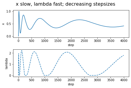
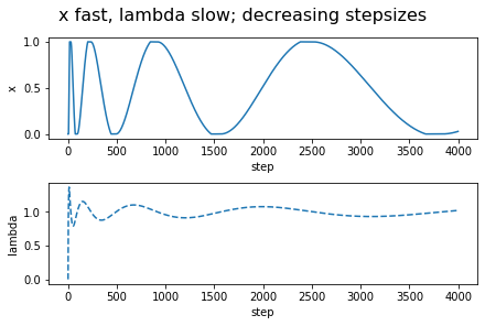
Interestingly, a simple Euler discretization, with decreasing step-sizes, one that is often used anyways when only a noisy "estimate" of the gradients $L_x'$ and $L_\lambda'$ are available, addresses all the concerns! We just have to think about the update of $\lambda$ being indefinitely faster than that of $x$, rather than thinking of $x$ being updated indefinitely slower than $\lambda$. This results in the updates \begin{align*} x_{k+1}-x_k &= - a_k (L_x'(x_k,\lambda_k)+W_k) \,,\\ \lambda_{k+1} - \lambda_k &= b_k (L_\lambda'(x_k,\lambda_k)+U_k)\,, \end{align*} where the positive stepsize sequences $(a_k)_k$, $(b_k)_k$ are such that $a_k \ll b_k$ and both converge to zero not too fast and not too slow, and where $W_k$ and $U_k$ are zero-mean noise sequences. This is what is known as a two-timescale stochastic approximation update. In particular, the timescale separation happens together with "convergence in the limit" if the stepsizes are chosen to satisfy \begin{align*} a_k = o(b_k) \quad k \to \infty\,,\\ \sum_k a_k = \sum_k b_k = \infty, \quad \sum_k a_k^2<\infty, \sum_k b_k^2 <\infty\,. \end{align*} This may make some worry about that $a_k$ will be too small and thus $x_k$ may converge slowly. The trick is to make $b_k$ larger rather than making $a_k$ smaller. For example, we can use $a_k = c/k$ if it is paired with $b_k = c/k^{0.5+\gamma}$ for $0<\gamma<0.5$. This makes the $\lambda_k$ iterates "more noisy", but the $x_k$ updates can smooth this noise out and since now $\lambda_k$ will also converge a little faster than usual, the $x_k$ can converge at the usual statistical rate of $1/\sqrt{k}$. The details are not trivial and a careful analysis is necessary to show that these ideas work and in fact I have not seen a complete analysis of this approach. To convince the reader that these ideas will actually work, I include a figure that shows how the iterates evolve in time in a simple, noiseless case. In fact, I include two figures: One when $x$ is updated on the slow timescale (the approach proposed here) but also the one when $\lambda$ is updated on the slow timescale. Surprisingly, this second approach is the one that makes an appearance in pretty much all the CMDP learning papers that use a two-timescale approach. As suggested by our argument of Part 3, and confirmed by the simulation results shown, this approach just cannot work: The $x$ variable will keep oscillating between its extreme values (representing deterministic policies).
|
|
If $x$ is the probability of taking the first action, the payoff under $r_0$ is $-x$ (e.g., $r_0(1)=-1$, $r_0(2)=0$). The payoff under $r_1$ is $x$ and the respective threshold is $0.5$. Altogether, this results in the constrained optimization problem "$\min_{x\in [0,1]} x$ subject to $x\ge 1/2$". The Lagrangian is $L(x,\lambda) = x + \lambda_*(1/2-x)$. The left-hand subfigure shows $x$ and $\lambda$ as a function of the number of updates when the stepsizes are $1/k$ ($1/\sqrt{k}$) for updating $x$ (respectively, $\lambda$). The stepsizes are reversed for the right-hand side figure. As it is obvious from the figures, only the variable that is updated on the slow timescale converges to its optimal value.
As the figures on the left-hand side attest, the algorithm works, though given how simple the example considered is, the oscillations and the slow convergence are rather worrysome. Readers familiar with the optimization literature will recognize this as a problem that has been long recognized in that literature, where various remedies have also been proposed. However, rather than exploring these here (for the curious reader, we give some pointers to the literature at the end of the post), let us turn to addressing the next major limitation of the approach presented so far, which is that in its current form the algorithm needs to maintain an occupancy measure over the states, which is usually quite problematic.
A trivial way to avoid representing occupancy measures is if search directly in a smoothly parameterized policy class. Let $\pi_\rho = \pi_\rho(a|s)$ be such a policy parameterization, where $\rho$ lives in some finite dimensional vector space. Then, we can write the Lagrangian \begin{align*} L(\rho,\lambda) & = - (1-\gamma) V^{\pi_\rho}(r_0,\mu) - \sum_i \lambda_i ((1-\gamma) V^{\pi_\rho}( r_i, \mu )-(1-\gamma)\theta_i) \\ & = - (1-\gamma) V^{\pi_\rho}\left(r_0+\sum_i \lambda_i r_i, \mu \right)+ (1-\gamma) \sum_i \lambda_i \theta_i\,, \end{align*} and our previous reasoning goes through without any changes. The gradient of $L$ with respect to $\rho$ can then be obtained using any of the "policy search" approaches available in the literature: As long as we can argue that these updates follow the gradient $L_\rho'(\rho,\lambda)$, we expect that the algorithm will find a locally optimal policy, which satisfies the value constraints.
Finally, to see what it takes to update the Lagrangian multipliers $(\lambda_i)_i$, we calculate \[ \frac{\partial}{\partial \lambda_i} L(\rho,\lambda) = (1-\gamma)\theta_i-(1-\gamma) V^{\pi_\rho}( r_i, \mu )\,. \] That is, $\lambda_i$ will be increased if the $i$th constraint is violated, while it will be decreased otherwise. Reassuringly, this makes intuitive sense. The update also tells us that the full algorithm will need to estimate the value of the policy to be updated under all the reward functions $r_i$.
Stepping back from the calculations a little, what saved the day here? Why could we reuse policy search algorithms to search for the solution of a constrained problem whereas in Part (4) we suggested that finding the optimal Lagrangian $\lambda^*$ and then solving the resulting minimization problem will not work? The magic is due to the use of gradient descent but the unsung hero is Danskin's theorem, which suggests that updating the parameters by following the partial derivative is a sensible choice.
Conclusions
As we saw, CMDPs are genuinely different from MDPs. Thus, if one faces a problem with value constraints, chances are good that the problem cannot be solved using techniques developed for MDPs alone. In particular, combining the rewards alone will be insufficient. As such, the reward hypothesis, appears to be limiting unless one in fact starts with a problem with no value constraints. However, we also saw that techniques developed for the single-objective case have the potential to be used in a more complicated setup where an outer loop optimizes the policy using a fixed linear combination of rewards, while an inner loop reoptimizes (on a faster timescale) the coefficients that combine the rewards. This latter finding implies that focusing on developing good methods for the single-objective case may have benefits even beyond the single-objective setting. Is this coincidence? I believe not. All in all, the story of the present post gives much needed ammunition to back a variant of the KISS principle applied to research:Priority should be given to developing a thorough understanding of simpler problems over working on more complex ones.
Of course, as any general arvice, this rule works also best when it is applied with moderation. In particular, the advice does not mean that we should never work on new problems, or that we should necessarily shy away from "big, hairy problems". Good research always dances on the boundary of what is possible.
As to specific research questions that one can ask, it appears that while there has been some work on developing algorithms for CMDPs, much remains to be done. Example of open questions include but are not limited to the following:
- Is there a strongly polynomial algorithm for finite CMDPs with a fixed discount factor?
- Prove that the two-timescale algorithm as proposed above indeed "works" (see notes on what results exist in this direction below).
- Can the two-timescale algorithm be made work for multiple discount factors? What changes?
- Get sample complexity results for the case when a simulator is available (say, with reset) and linear function approximation is used to estimate value functions.
- Design efficient exploration methods for CMDPs, with or without function approximation (the notes again list existing results).
- Design efficient algorithms for the batch version of the CMDP problem.
Notes (bibliographical and other)
- Uniform optimality can be defined either with respect to initial states (a policy is uniformly optimal if it is optimal no matter the initial state), or with respect to initial state distributions. The latter is the definition I used in this post. For brevity, call the former S-uniform optimality, the latter D-uniform optimality. Clearly, if a policy is D-uniformly optimal then it is also S-uniformly optimal (starting from a fixed state $s$ corresponds to choosing a special initial state distribution which assigns probability one to state $s$). The reverse does not hold, as attested by the two-state CMDP described in Part (1): In this MDP, there is an S-uniformly optimal stationary policy ($\pi^*$), while, there is no D-uniformly optimal stationary policy. It is not hard to construct MDPs where the set of S-uniformly optimal stationary policies is also empty.
- As noted earlier, the basic reference to constrained MDPs is the book of Eitman Altman. The first part of this post is based partly on Chapters 2 and 3 of this book.
- One of my favorite pet topics is hunting for examples where randomness (probabilities) provably "helps". As an example of a problem where I don't think we have a clear understanding of whether stochasticity helps is when we build world models for the purpose of control (again, there should perhaps be a post about why we like to think of the world as an MDP). The canonical example of where randomization provably helps is simultaneous action games (like rock-paper-scissors). In this post we saw that CMDPs provide another simple example: The appeal of this is that this example does not even need two agents. Of course, given what we now know about CMDPs and games, the two examples are not quite independent.
- So in Part (1) we established that randomization is essential. But "how much" randomization does one need? It turns out that one can show that in any finite CMDP there always exists an optimal stationary policy $\pi^*$ such that $R(\pi^*):=\sum_s |\text{supp}(\pi^*(\cdot|s))|$ is at most $|S|+n$. Here, $|\text{supp}(\pi^*(\cdot|s))|$ is the number of nonzero values that $\pi(\cdot|s)$ takes. Note that if $\pi^*$ was deterministic, then $R(\pi^*)$ would be $|S|$. It follows that in a CMDP with $n$ constraints, one can always find a stationary policy that randomizes only at $n$ or fewer states. This result is stated in Chapter 3 of Altman's book.
- The hardness results are taken from a paper of Eugene Feinberg. This paper also mentions some previous hardness results. For example, it mentions a result of Filar and Krass from 1994 that states that computing the best deterministic policy for a constrained unichain MDP with average rewards per unit time is also NP-hard. It also considers the so-called weighted discounted criteria where the goal is to maximize $\sum_i w_i V^\pi(r_i,\gamma_i,\mu)$ where $V^\pi(r_i,\gamma_i,\mu)$ stands for the total expected reward under $r_i$ and $\pi$ with start distribution $\mu$ and discount factor $\gamma_i$ (the original reference to these problems is Feinberg and Shwartz from 1994 and 95). These problems are quite different to CMDPs. For example, stationary policies are in general not sufficient for these problems. Based on the theorem cited in this post, Feinberg in his paper shows the hardness of finding a feasible stationary policy in such weighted discounted MDPs.
- Unsurprisingly, multicriteria Markovian Decision Processes are a common topic in the AI/CS literature. A relatively recent survey by Roijers et al., just like this post, is also aimed at explaining the relationship between multi- and single-objective problems. This paper also starts from the reward hypothesis and postulates that this hypothesis implies that one should be able to convert any multiobjective MDP into a single-objective one in a two-step process. In the first step, the multiple value functions are combined by the help of a "scalarization function" a single value function, while in the second step one should find an MDP such that for all policies, the value function of the policy is equal to the "scalarized" value function of that policy (this means the new MDP must have the same policies, hence, same state and action space). This appears to me a rather specific interpretation of the reward hypothesis. The reader who got to this point in the post will not be surprised to learn that the Roijers et al.' main point is that this scalarization will hardly ever work.
- The constructive part of this paper is concerned with the construction of coverage sets; a generalization of Pareto optimality. The coverage set construction problem is as follows: One is given a family $\mathcal{F}$ of so-called scalarization functions of the form $f: \mathbb{R}^n \to \mathbb{R}$. Given $f\in \mathcal{F}$, solving the $f$-scalarized problem means finding a policy $\pi$ that maximizes $f(V^\pi(r_1,\mu),\dots,V^\pi(r_n,\mu))$. Call the resulting policy $f$-optimal. A coverage set is a subset $\Pi$ of all policies, such that no matter what scalarizer $f\in \mathcal{F}$ is chosen, one can always find an $f$-optimal policy in $\Pi$. The goal is to find a minimal coverage set. A relaxed version of the problem is to find $\Pi$ so that for any $f\in \mathcal{F}$, an $f$-optimal policy can be computed from $\Pi$ efficiently. For example, if $\mathcal{F}$ contains linear functions with "weights" from a nonempty set $W \subset \mathbb{R}^n$, it suffices to compute optimal policies for the extrema of $W$: A "convex" interpolation (randomizing over elements in $\Pi$) is then sufficient to reconstruct any optimal policy. While this is interesting, it is unclear what user would be happy with such randomizing solutions.
- Constraints that rule out visiting states can be incorporated in the CMDP framework by introducing a reward that takes on $-1$ at the forbidden states and $0$ otherwise, setting both the discount factor associated with this reward, and the respective threshold to zero. This example underlines the importance of studying the case when there are multiple distinct discount factors.
- Constraints can also be enforced by adding a safety filter: In this approach, actions of the policy are not sent to the environment, but are sent to the "safety filter" which modifies them as needed. This allows one to concentrate on one problem at a time: The environment together with the "box" that implements the safety filter becomes the new environment where one only needs to be concerned with maximizing value. The burden is then on designing the "safety filter". This is a classical approach. In a recent talk, which I can only warmly recommend, Melanie Zeilinger explored the problem of using learning to design better safety filters. Another recent work on designing safety filters by my colleagues at DeepMind is based on a local linearization approach.
- A pioneer of the Lagrangian approach to learning to act in CMDPs is Vivek S. Borkar. Incidentally, and not accidantally, Borkar is also one of the main characters behind two-timescale stochastic approximation. (His short book on stochastic approximation is a true gem!) In his paper, Borkar considers finite CMDPs. He proposes to update the Lagrangian multipliers on the slow timescale, which, as we saw in Part 4, cannot guarantee convergence of the policy to the optimal solution (although, after Theorem 4.1, Borkar suggests otherwise). A similar approach is followed in the concurrent paper of Vikram Krishnamurthy, Katerina Martin and Felisa Vázquez-Abad, who also explore an algorithm similar to the use of augmented Lagrangians, which may fix these issues. In his paper, Borkar uses the envelope theorem (often used in economics) to argue for the convergence of the Lagrangian multipliers to their optimal value. In simple cases, this theorem essentially follows from Danskin's theorem applied to the Lagrangian of the constrained optimization problem. The stronger versions of the envelope theorem are useful in that they do not need the differentiability of the value function $\Phi$ which often fails to hold. A more recent paper by Shalabh Bhatnagar and K. Lakshmanan generalizes the approach of Borkar to the case when function approximators are used. The guarantees get correspondingly weaker. The work of Chen Tessler, Daniel Makowitz and Shie Mannor allows for general path dependent constraints. Besides this, the main contribution in this paper is allowing nonlinearly parameterized value functions and policies. Just like the previously mentioned works, curiously, the slow timescale is still used for updating the Lagrangian multipliers. One reason that I can see for this choice is that this allows both a simpler analysis and a straightforward reuse of all existing algorithms developed for MDPs (on the fast timescale), while if the MDP algorithm needs to work on the slow timescale then one is forced to use a "gradient-like" algorithm and a more complicated analysis needs to be developed.
- Other early work on multi-objective RL includes that of Shie Mannor and Nahum Shimkin who consider the more general problem of learning policies (even in the presence of adversaries) that steer the average reward of a vector-valued reward function into a set of the user's choice. The algorithms here are based on Blackwell's approachability theorem which says that multiple objectives can be satisfied simultaneously in an adversarial environment if and only if they can be satisfied in a stochastic one with a known law. Mannor and Shimkin use this result then to create algorithms for multi-criteria MDPs for "steering" the objectives into some set that the user should specify.
- The paper of my colleagues at DeepMind, which was also mentioned at the beginning, gives an example when the Lagrangian approach is combined with RL algorithms that use neural networks. This paper replaces the policy update of Tessler et al. with a mirror-descent like update, which underlies the RL algorithm known as MPO. The authors of this paper noted that the algorithm can be highly unstable (see the figures above). As a remedy, they propose heuristic techniques such as normalizing the Lagrangian multipliers and reparameterizing them to keep them nonnegative. The authors also suggest to impose constraints with respect to many initial states (or distributions) simultaneously. To facilitate this, a neural network is used to predict the Lagrangians (the input to the network is the state from where the constraint should hold). With these extra constraints, one may need to add memory to the policies to avoid losing too much on performance. They also suggest to consider a parameterized version of the CMDP problem where the value constraint thresholds are included as parameters. To reduce the computational cost of solving many instances and to generalize existing solutions to new values of these thresholds, they feed the thresholds as inputs to the neural networks. A pleasent side-effect of this is that the oscillations are reduced. The approach is illustrated on several robotic tasks, where task success rate is constrained and control cost (in terms of energy) is minimized. An alternative to this approach, is the earlier work of Achiam et al. who present an approach based on conservative policy iteration (and TRPO). Their problem setting is harder: Their goal is to maintain the constraints even during learning. Perhaps another blog should discuss the merits and limits of both MPO and TRPO (and related approaches).
- When we use a policy parameterisation, the objective $L$ becomes nonconvex-concave. In this case, the two-timescale approach still works. In a recent paper, Chi Jin and co-workers derived finite time results on the rate of convergence of this method to a local optima who point out that in game-theory terms, the solution of the min-max problem corresponds to a (local) Stackelberg equilibrium, rather than a Nash equilibrium. It was mentioned before that instability of solving the minmax problem that arises from the Lagrangian approach is widely recognized in the optimization community. To stabilize the min-max solvers, a standard recommendation is to add a small penalty that penalizes constraint violations, resulting in the so-called augmented Lagrangian method. Averaging is another tool that is often used (on the top of, for example, a gradient algorithm). As it was mentioned earlier, the early paper of Krishnamurty et al. already explored this idea. A nice little paper by my former PhD student Yaoliang Yu and his student Guojun Zhang explores the (mis)behavior of gradient methods in bilinear problems, like the ones we have seen here. In another nice paper, the nonlinear min-max problem is looked at by the same team expanded with Pascal Poupart. The literature on min-max problems or solving constrained problems is huge -- so I need to stop here.
- Provably efficient learning to solve a CMDP recently became a hot topic. Liyuan Zheng and Lillian J. Ratliff considered known transitions and rewards and the average reward criterion, and a known initial safe exploration policy. The UCRL2 algorithm is modified and it is assumed that the underlying controlled Markov chain has a finite diameter. The authors prove $O(T^{3/4})$ high probability regret up to log factors for the rewards from $r_0$ while they also show that the policies chosen satisfy the constraints with high probability at all time steps. (This seems to generalize "conservative bandits", which we explored with my group a while back.) The paper of Efroni, Mannor and Pirotta gives a nice overview of related work (including work on budgeted bandits, safe exploration and more). They consider the significantly easier finite horizon setting, but the problem is made more challenging because the transition structure is no longer assumed to be known. They give algorithms (also based on optimism) for which they show that both the regret with respect to the reward to be maximized and the constraints are controlled sublinearly (essentially, $\sqrt{T}$ is achieved). The concurrent work of Qui et al. also considers this case, but with adversarially chosen rewards (both for the main objective and the constraints). Ding et al. again considered the finite horizon setting, the so-called linear MDP case where linear function approximation is used. They gave similar results to the previous paper.
References
- Eitan Altman: Constrained Markov Decision Processes, CRC Press, 2000. Free pdf
- Eugene Feinberg: Constrained Discounted Markov Decision Process and Hamiltonian Cycles, MOR, 25:1, 2000. Free pdf from the author's homepage.
- Diederik M Roijers, Peter Vamplew, Shimon Whiteson, and Richard Dazeley: A Survey of Multi-Objective Sequential Decision-Making, JAIR, 2013.
- Borkar, V. S. An Actor-Critic Algorithm for Constrained Markov Decision Processes, Systems and Control Letters 54 (3): 207--213, 2005.
- Krishnamurthy, V., K. Martin, and F. Vasquez Abad. Implementation of Gradient Estimation to a Constrained Markov Decision Problem, In 42nd IEEE International Conference on Decision and Control, 2003. Repost to arXiv from 2008, with two authors.
- Mannor, Shie, and Nahum Shimkin, A Geometric Approach to Multi-Criterion Reinforcement Learning, Journal of Machine Learning Research: JMLR 5: 325-360, 2004.
- Bhatnagar, Shalabh, and K. Lakshmanan, An Online Actor–Critic Algorithm with Function Approximation for Constrained Markov Decision Processes. Journal of Optimization Theory and Applications 153 (3): 688–708, 2012.
- Lin, Tianyi, Chi Jin, and Michael I. Jordan. On Gradient Descent Ascent for Nonconvex-Concave Minimax Problems, June, 2019, arXiv.
- Zheng, Liyuan, and Lillian J. Ratliff. Constrained Upper Confidence Reinforcement Learning, arXiv 2020.
- Efroni, Yonathan, Shie Mannor, and Matteo Pirotta. Exploration-Exploitation in Constrained MDPs, arXiv 2020.
- Qiu, Shuang, Xiaohan Wei, Zhuoran Yang, Jieping Ye, and Zhaoran Wang. Upper Confidence Primal-Dual Optimization: Stochastically Constrained Markov Decision Processes with Adversarial Losses and Unknown Transitions arXiv 2020.
- Ding, Dongsheng, Xiaohan Wei, Zhuoran Yang, Zhaoran Wang, and Mihailo R. Jovanović. Provably Efficient Safe Exploration via Primal-Dual Policy Optimization, arXiv 2020.
- Bohez, Steven, Abbas Abdolmaleki, Michael Neunert, Jonas Buchli, Nicolas Heess, and Raia Hadsell. Value Constrained Model-Free Continuous Control, February, arXiv 2019.
- Tessler, Chen, Daniel J. Mankowitz, and Shie Mannor. Reward Constrained Policy Optimization, ICLR, January, 2019.
- Achiam, Joshua, David Held, Aviv Tamar, and Pieter Abbeel. Constrained Policy Optimization, ICML, 2017.
- Zhang, Guojun, and Yaoliang Yu. 2019/20: Convergence of Gradient Methods on Bilinear Zero-Sum Games, March, 2020.
- Zhang, Guojun, Pascal Poupart, and Yaoliang Yu. 2020. Optimality and Stability in Non-Convex-Non-Concave Min-Max Optimization, February, 2020
- Dalal, Gal, Krishnamurthy Dvijotham, Matej Vecerik, Todd Hester, Cosmin Paduraru, and Yuval Tassa. Safe Exploration in Continuous Action Spaces, arXiv, 2018.
Hello! I'm trying to credit the author of this blog, but I can't actually find any information about who's website this is. This may be anonymous, but if not, can you let me know who you are? Perhaps with a reply comment? :D
ReplyDeleteThis is the author, Csaba Szepesvari. It's funny that I optimized away any information about myself. Well, everything for a more pleasant look:)
ReplyDeleteThanks Csaba for an excellent post on constrained or in general MO MDPs and the perils of scalarization. The industry is moving towards MDP setting with long term objective(s) in mind and there is no single objective that we wish to optimize over the horizon. This post clearly articulates why this is a tough problem, why some simple techniques may be sub-optimal and provides excellent literature on where to look for more ideas.
ReplyDeleteIt is so well-organized and solid. Thanks a lot!
ReplyDeleteThanks for the great post, super interesting!
ReplyDeleteQuick question: where does the (1 - \gamma) factor comes from in the last set of equations (between the plots and the Conclusion). I understand that this factor appeared to normalise the occupancy measure earlier, but at the end since you rewrite the Lagrangian using value functions rather than occupancy measures (directly from your initial CMDP definition) I don't see how 1-\gamma got in there? Thanks!
@Julien: Thanks for your comments. Indeed, there were some typos, which I have now corrected. The relationship is that (1-gamma)*value = , and I missed some (1-gamma) factors. At the end, the (1-gamma) factor appears in all the terms, and could be removed without changing anything. I left them there because they don't matter anyways and this way we can just reuse the same Lagrangian function that we had before with an equality.
ReplyDelete